
[vc_row][vc_column][vc_wp_text]
[xyz-ips snippet=”metadatatitle”]
[/vc_wp_text][vc_empty_space][/vc_column][/vc_row][vc_row][vc_column width=”2/3″][vc_column_text]
To date, most industrial process data is fed to proprietary SCADA systems that are great at what they do — monitor and control industrial processes. What if a business entity wanted to work more closely with their business and IT teams that aren’t familiar with SCADA software? The disconnect between IT and OT software systems is slowly being bridged, but there aren’t many options to solve this problem to date. By bridging these systems, businesses are lowering costs, improving efficiencies, and generating new value for their customers. Big data is a buzz word used to describe one of the key technologies helping to bridge this data gap. These technologies are a key component of next generation industrial systems because of the amount of data which industrial processes can generate in real time. In this article, I’ll provide a concrete way to get industrial data out of the proprietary world, and into big data systems which IT and business teams can start to leverage.
This article is intended to provide documentation on one specific application which integrates industrial process data into a modern big data platform. This how-to is focused on one of the most popular big data platforms, Elasticsearch (‘ELK’ stack). To integrate the sensor data into Elasticsearch, Logstash was used. The visualization tool Kibana was used to perform basic visualization and data analysis. To collect the data from the process devices and sensors, the PDR 1000 from Phoenix Contact was integrated. By the end of this guide, you will be applying Machine Learning to an industrial process. Through this process, we’ll gain insight into how big data technologies can be applied to industrial processes and what new value might be gained.
[/vc_column_text][vc_empty_space][vc_column_text]
What is Elasticsearch?
[/vc_column_text][vc_empty_space][vc_column_text] [/vc_column_text][vc_empty_space][vc_column_text]
Elasticsearch is a ‘big data’ database and search engine. It excels at scaling, hence the name Elastic. It is able to handle very large data sets in terms of the quantity of data stored, the speed of collection and the distribution of this data. Elasticsearch supports data redundancy and integrity across large numbers of supporting nodes (‘computers’). With Docker support, it is easily deployed in the cloud, in a server room, or on an industrial computer. These features make it a great candidate for industrial applications and lends itself well to merging IT and OT operating metrics.
Perhaps it’s best feature, a built in HTTP API allows web applications and custom computer applications to be easily integrated. If you’re a developer, I highly recommend checking out the Elasticsearch website for integration ideas.
Being based on open source software and therefore free*, Elasticsearch is used across industries to build advanced tools to improve their businesses and provide additional value to their customers. There are many great application examples and use cases for Elasticsearch. For brevity, I’ll put a link to their website and customer application references.
*Elasticsearch is free for basic use cases, but requires a license for advanced features. More info here
[/vc_column_text][vc_empty_space][vc_column_text]
What is Kibana?
[/vc_column_text][vc_empty_space][vc_column_text]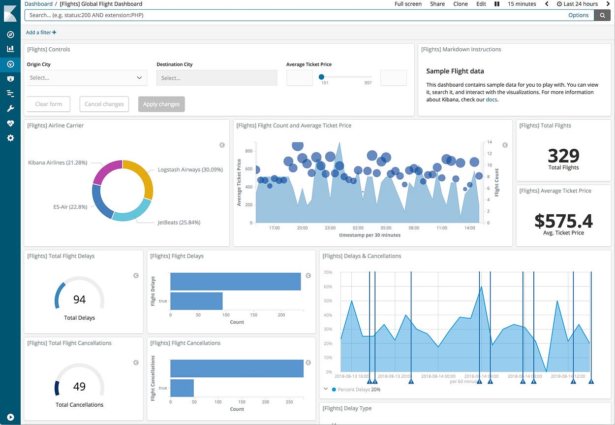 [/vc_column_text][vc_empty_space][vc_column_text]
Kibana is a user interface which allows Elasticsearch users to visualize and analyze their data quickly. Similar in functionality to most industrial SCADA analytics systems, it includes many tools for creating data visualizations. With the 30 day trial license, Kibana can be used to generate Machine Learning tests, generate alerts, create reports and enable more advanced features like integrated network security.
[/vc_column_text][vc_empty_space][vc_column_text]
What is Logstash?
[/vc_column_text][vc_empty_space][vc_column_text]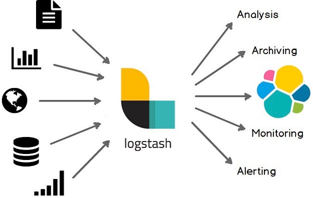 [/vc_column_text][vc_empty_space][vc_column_text]
Logstash is an application written to ‘ship’ data to Elasticsearch. It provides 3 main functions and provides various plugins for these functions -> Data Collection/Input -> Data Processing -> Data Output. Though Logstash was built for Elasticsearch, it has the ability to provide data to other services via output plugins. A few of the more interesting output plugins for industrial applications are listed below as of Logstash version 7.4. Here is a link to the full list.
- CSV — convert data to a CSV file
- Email — sends an email when certain input conditions are met
- Kafka — sends data to the Kafka big data messaging system
- Mongodb — noSQL, very popular, and modern noSQL database
- Redis — high performance, RAM based database
- InfluxDB— multithreaded, high performance database
[/vc_column_text][vc_empty_space][vc_column_text]
The Hardware — PDR 1000
[/vc_column_text][vc_empty_space][vc_column_text]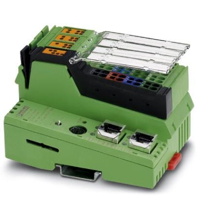 [/vc_column_text][vc_empty_space][vc_column_text]
The PDR 1000 is an industrial IoT data collector. It is great for monitoring industrial process data with a wide operating temperature range: -25 deg C (-13 F) to 55 deg. C (131 F ). Industrial sensors can be integrated easily with analog, digital, temperature sensors and Modbus TCP support. The built in web interface makes configuration and monitoring a breeze.
[/vc_column_text][vc_empty_space][vc_column_text] [/vc_column_text][vc_empty_space][vc_column_text]
Getting into it
[/vc_column_text][vc_empty_space][vc_column_text]
Now that we’ve done a brief description of the different components used in this demo, let’s review the basic architecture.
[/vc_column_text][vc_empty_space][vc_column_text]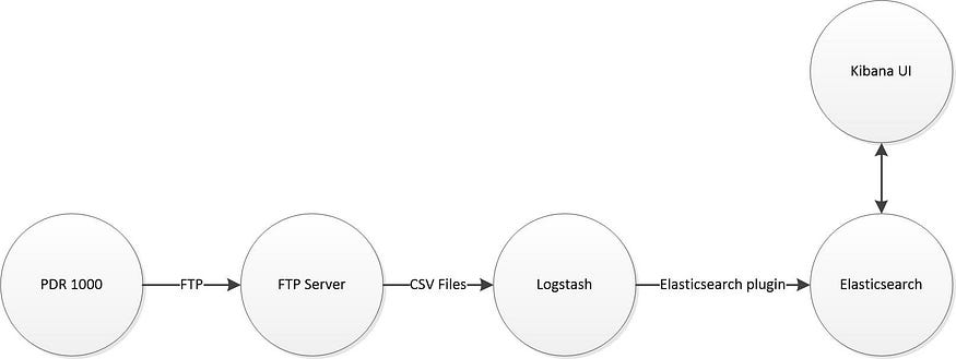 [/vc_column_text][vc_empty_space][vc_column_text]
Some assumptions made about your setup:
- You have Elasticsearch, Logstash, and Kibana installed. Click the links for the download and install instructions
- You have an FTP server set up. For this demo, a simple FileZilla server was used.
PDR Setup
The PDR 1000 is very easy to get set up to monitor industrial sensor data and collect data from Modbus data providers such as the Radioline 900 IFS. We’ll start by aggregating and recording this data using the PDR.
First, connect to the PDR using http://[ip address of pdr]. When it finishes connecting, the PDR IO modules will need to be selected and then the home screen is displayed.
[/vc_column_text][vc_empty_space][vc_column_text]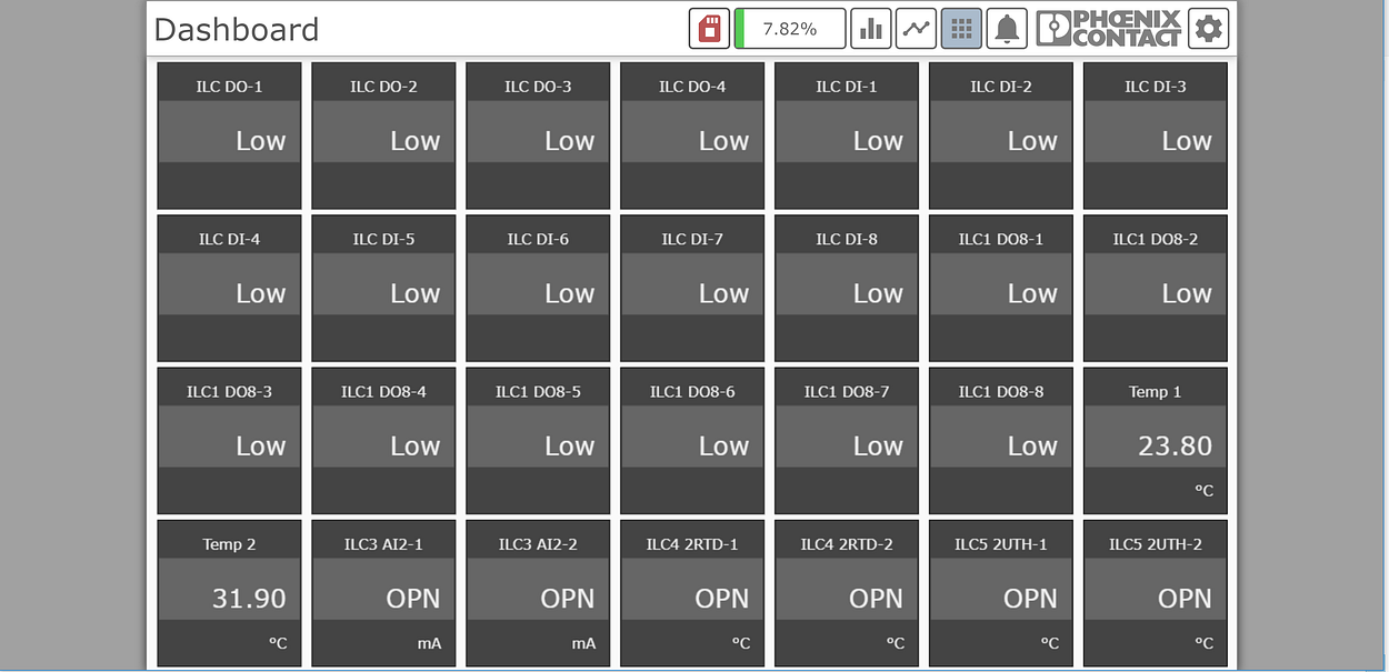 [/vc_column_text][vc_empty_space][vc_column_text]
My PDR for this example project has a few digital inputs, outputs, analog inputs (AI), Thermocouple inputs (UTH) and RTD temperatures sensors (RTD). To configure the name of the data points and reconfigure them, click on the gear icon in the top right of the screen.
[/vc_column_text][vc_empty_space][vc_column_text]
You will need to log in in order to access these pages. The default password for the root user is private. Please make sure to change this password after the first log in.
After logging in, you will be taken to the IO configuration page. On the left, the IO channel can be selected and the associated configuration parameters can be changed. For this example project, I had two active thermocouple inputs that I renamed ‘Temp 1’ and ‘Temp 2.’ I left their default configuration options in degrees Centigrade.
[/vc_column_text][vc_empty_space][vc_column_text] [/vc_column_text][vc_empty_space][vc_column_text]
After configuring the IO, I set up the PDR’s FTP feature by clicking the hamburger button in the top right and selecting settings.
[/vc_column_text][vc_empty_space][vc_column_text]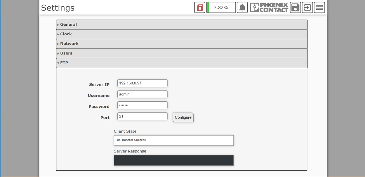 [/vc_column_text][vc_empty_space][vc_column_text]
Put in the settings of your FTP server and click configure. By default, FTP uses port 21, but can be modified here.
The final step to begin logging and transferring data is to configure recording. This is performed on the recording page. Navigate to this page via the hamburger button on the top right of the web page.
[/vc_column_text][vc_empty_space][vc_column_text] [/vc_column_text][vc_empty_space][vc_column_text]
Drag and drop the channels to be recorded onto the ‘Recorded I/O’ drop area. Then, use the basic settings to configure the logging rate. In order to have your data pushed via the FTP system, you must enable CSV file logging here. Now, once an hour, my PDR will push a CSV file of my logged data to the FTP server configured earlier.
Logstash Setup
Once the CSV files are located on a host machine as defined in and output from the FTP server, we can start up Logstash with the example configuration file below written to parse the PDR data. It will handle any metric name and will also send events to Elasticsearch for sensor or Modbus errors. In this way,our Elasticsearch application will be able to identify times when the end device was not working as expected.
A few notes on this config file which was written for Windows
- sincedb_path must be set to “NUL” for Windows
- “path” key must contain forward slashes on Windows e.g. C:/Users/guest/Downloads/pdr*.csv
[/vc_column_text][vc_empty_space][vc_raw_html]JTNDcHJlJTIwY2xhc3MlM0QlMjJodSUyMGh2JTIwaHclMjBoeCUyMGh5JTIwbXQlMjBtdSUyMG12JTIyJTNFJTNDc3BhbiUyMGlkJTNEJTIyNWI4MCUyMiUyMGNsYXNzJTNEJTIyYXAlMjBqeiUyMGthJTIwY2clMjBtdyUyMGIlMjBnbCUyMG14JTIwbXklMjByJTIwbXolMjIlMjBkYXRhLXNlbGVjdGFibGUtcGFyYWdyYXBoJTNEJTIyJTIyJTNFaW5wdXQlMjAlN0IlM0MlMkZzcGFuJTNFJTNDc3BhbiUyMGlkJTNEJTIyMDEwYyUyMiUyMGNsYXNzJTNEJTIyYXAlMjBqeiUyMGthJTIwY2clMjBtdyUyMGIlMjBnbCUyMG5hJTIwbmIlMjBuYyUyMG5kJTIwbmUlMjBteSUyMHIlMjBteiUyMiUyMGRhdGEtc2VsZWN0YWJsZS1wYXJhZ3JhcGglM0QlMjIlMjIlM0UlMjBmaWxlJTIwJTdCJTNDJTJGc3BhbiUzRSUzQ3NwYW4lMjBpZCUzRCUyMmUyN2UlMjIlMjBjbGFzcyUzRCUyMmFwJTIwanolMjBrYSUyMGNnJTIwbXclMjBiJTIwZ2wlMjBuYSUyMG5iJTIwbmMlMjBuZCUyMG5lJTIwbXklMjByJTIwbXolMjIlMjBkYXRhLXNlbGVjdGFibGUtcGFyYWdyYXBoJTNEJTIyJTIyJTNFJTIwJTIwcGF0aCUyMCUzRCUyNmd0JTNCJTIwJTIyJTVCeW91ciUyMGZ0cCUyMGRvd25sb2FkcyUyMHBhdGglMjBoZXJlJTVEJTJGcGRyJTJBLmNzdiUyMiUzQyUyRnNwYW4lM0UlM0NzcGFuJTIwaWQlM0QlMjI5YTJiJTIyJTIwY2xhc3MlM0QlMjJhcCUyMGp6JTIwa2ElMjBjZyUyMG13JTIwYiUyMGdsJTIwbmElMjBuYiUyMG5jJTIwbmQlMjBuZSUyMG15JTIwciUyMG16JTIyJTIwZGF0YS1zZWxlY3RhYmxlLXBhcmFncmFwaCUzRCUyMiUyMiUzRSUyMCUyMHN0YXJ0X3Bvc2l0aW9uJTIwJTNEJTI2Z3QlM0IlMjAlMjJiZWdpbm5pbmclMjIlM0MlMkZzcGFuJTNFJTNDc3BhbiUyMGlkJTNEJTIyNGE5ZCUyMiUyMGNsYXNzJTNEJTIyYXAlMjBqeiUyMGthJTIwY2clMjBtdyUyMGIlMjBnbCUyMG5hJTIwbmIlMjBuYyUyMG5kJTIwbmUlMjBteSUyMHIlMjBteiUyMiUyMGRhdGEtc2VsZWN0YWJsZS1wYXJhZ3JhcGglM0QlMjIlMjIlM0UlMjAlMjBzaW5jZWRiX3BhdGglMjAlM0QlMjZndCUzQiUyMCUyMk5VTCUyMiUzQyUyRnNwYW4lM0UlM0NzcGFuJTIwaWQlM0QlMjJjMDU3JTIyJTIwY2xhc3MlM0QlMjJhcCUyMGp6JTIwa2ElMjBjZyUyMG13JTIwYiUyMGdsJTIwbmElMjBuYiUyMG5jJTIwbmQlMjBuZSUyMG15JTIwciUyMG16JTIyJTIwZGF0YS1zZWxlY3RhYmxlLXBhcmFncmFwaCUzRCUyMiUyMiUzRSUyMCU3RCUzQyUyRnNwYW4lM0UlM0NzcGFuJTIwaWQlM0QlMjIzZGMxJTIyJTIwY2xhc3MlM0QlMjJhcCUyMGp6JTIwa2ElMjBjZyUyMG13JTIwYiUyMGdsJTIwbmElMjBuYiUyMG5jJTIwbmQlMjBuZSUyMG15JTIwciUyMG16JTIyJTIwZGF0YS1zZWxlY3RhYmxlLXBhcmFncmFwaCUzRCUyMiUyMiUzRSU3RCUzQyUyRnNwYW4lM0UlM0NzcGFuJTIwaWQlM0QlMjI1NThhJTIyJTIwY2xhc3MlM0QlMjJhcCUyMGp6JTIwa2ElMjBjZyUyMG13JTIwYiUyMGdsJTIwbmElMjBuYiUyMG5jJTIwbmQlMjBuZSUyMG15JTIwciUyMG16JTIyJTIwZGF0YS1zZWxlY3RhYmxlLXBhcmFncmFwaCUzRCUyMiUyMiUzRWZpbHRlciUyMCU3QiUzQyUyRnNwYW4lM0UlM0NzcGFuJTIwaWQlM0QlMjI3NWRkJTIyJTIwY2xhc3MlM0QlMjJhcCUyMGp6JTIwa2ElMjBjZyUyMG13JTIwYiUyMGdsJTIwbmElMjBuYiUyMG5jJTIwbmQlMjBuZSUyMG15JTIwciUyMG16JTIyJTIwZGF0YS1zZWxlY3RhYmxlLXBhcmFncmFwaCUzRCUyMiUyMiUzRSUyMGNzdiUyMCU3QiUzQyUyRnNwYW4lM0UlM0NzcGFuJTIwaWQlM0QlMjJjOGZjJTIyJTIwY2xhc3MlM0QlMjJhcCUyMGp6JTIwa2ElMjBjZyUyMG13JTIwYiUyMGdsJTIwbmElMjBuYiUyMG5jJTIwbmQlMjBuZSUyMG15JTIwciUyMG16JTIyJTIwZGF0YS1zZWxlY3RhYmxlLXBhcmFncmFwaCUzRCUyMiUyMiUzRSUyMCUyMHNlcGFyYXRvciUyMCUzRCUyNmd0JTNCJTIwJTIyJTJDJTIyJTNDJTJGc3BhbiUzRSUzQ3NwYW4lMjBpZCUzRCUyMmM5ZDclMjIlMjBjbGFzcyUzRCUyMmFwJTIwanolMjBrYSUyMGNnJTIwbXclMjBiJTIwZ2wlMjBuYSUyMG5iJTIwbmMlMjBuZCUyMG5lJTIwbXklMjByJTIwbXolMjIlMjBkYXRhLXNlbGVjdGFibGUtcGFyYWdyYXBoJTNEJTIyJTIyJTNFJTIwJTIwYXV0b2RldGVjdF9jb2x1bW5fbmFtZXMlMjAlM0QlMjZndCUzQiUyMHRydWUlM0MlMkZzcGFuJTNFJTNDc3BhbiUyMGlkJTNEJTIyMjY1MSUyMiUyMGNsYXNzJTNEJTIyYXAlMjBqeiUyMGthJTIwY2clMjBtdyUyMGIlMjBnbCUyMG5hJTIwbmIlMjBuYyUyMG5kJTIwbmUlMjBteSUyMHIlMjBteiUyMiUyMGRhdGEtc2VsZWN0YWJsZS1wYXJhZ3JhcGglM0QlMjIlMjIlM0UlMjAlN0QlM0MlMkZzcGFuJTNFJTNDc3BhbiUyMGlkJTNEJTIyNDQxMiUyMiUyMGNsYXNzJTNEJTIyYXAlMjBqeiUyMGthJTIwY2clMjBtdyUyMGIlMjBnbCUyMG5hJTIwbmIlMjBuYyUyMG5kJTIwbmUlMjBteSUyMHIlMjBteiUyMiUyMGRhdGEtc2VsZWN0YWJsZS1wYXJhZ3JhcGglM0QlMjIlMjIlM0UlMjBkYXRlJTIwJTdCJTNDJTJGc3BhbiUzRSUzQ3NwYW4lMjBpZCUzRCUyMjdlNzYlMjIlMjBjbGFzcyUzRCUyMmFwJTIwanolMjBrYSUyMGNnJTIwbXclMjBiJTIwZ2wlMjBuYSUyMG5iJTIwbmMlMjBuZCUyMG5lJTIwbXklMjByJTIwbXolMjIlMjBkYXRhLXNlbGVjdGFibGUtcGFyYWdyYXBoJTNEJTIyJTIyJTNFJTIwJTIwbWF0Y2glMjAlM0QlMjZndCUzQiUyMCU1QiUyMlRpbWVzdGFtcCUyMiUyQyUyMllZWVklMkZNTSUyRmRkJTIwSEglM0FtbSUzQXNzJTIyJTJDJTIyWVlZWSUyRk1NJTJGZGQlMjBISCUzQW1tJTNBc3MuU1NTJTIyJTJDJTIySVNPODYwMSUyMiU1RCUzQyUyRnNwYW4lM0UlM0NzcGFuJTIwaWQlM0QlMjJjOWI0JTIyJTIwY2xhc3MlM0QlMjJhcCUyMGp6JTIwa2ElMjBjZyUyMG13JTIwYiUyMGdsJTIwbmElMjBuYiUyMG5jJTIwbmQlMjBuZSUyMG15JTIwciUyMG16JTIyJTIwZGF0YS1zZWxlY3RhYmxlLXBhcmFncmFwaCUzRCUyMiUyMiUzRSUyMCU3RCUzQyUyRnNwYW4lM0UlM0NzcGFuJTIwaWQlM0QlMjJjODViJTIyJTIwY2xhc3MlM0QlMjJhcCUyMGp6JTIwa2ElMjBjZyUyMG13JTIwYiUyMGdsJTIwbmElMjBuYiUyMG5jJTIwbmQlMjBuZSUyMG15JTIwciUyMG16JTIyJTIwZGF0YS1zZWxlY3RhYmxlLXBhcmFncmFwaCUzRCUyMiUyMiUzRSUyMHJ1YnklMjAlN0IlM0MlMkZzcGFuJTNFJTNDc3BhbiUyMGlkJTNEJTIyOGQyNCUyMiUyMGNsYXNzJTNEJTIyYXAlMjBqeiUyMGthJTIwY2clMjBtdyUyMGIlMjBnbCUyMG5hJTIwbmIlMjBuYyUyMG5kJTIwbmUlMjBteSUyMHIlMjBteiUyMiUyMGRhdGEtc2VsZWN0YWJsZS1wYXJhZ3JhcGglM0QlMjIlMjIlM0UlMjAlMjBjb2RlJTIwJTNEJTI2Z3QlM0IlMjAlMjIlM0MlMkZzcGFuJTNFJTNDc3BhbiUyMGlkJTNEJTIyMjJhMSUyMiUyMGNsYXNzJTNEJTIyYXAlMjBqeiUyMGthJTIwY2clMjBtdyUyMGIlMjBnbCUyMG5hJTIwbmIlMjBuYyUyMG5kJTIwbmUlMjBteSUyMHIlMjBteiUyMiUyMGRhdGEtc2VsZWN0YWJsZS1wYXJhZ3JhcGglM0QlMjIlMjIlM0UlMjAlMjAlMjBldmVudC50b19oYXNoLmVhY2glMjAlN0IlMjAlN0NrJTJDJTIwdiU3QyUzQyUyRnNwYW4lM0UlM0NzcGFuJTIwaWQlM0QlMjJhNmMxJTIyJTIwY2xhc3MlM0QlMjJhcCUyMGp6JTIwa2ElMjBjZyUyMG13JTIwYiUyMGdsJTIwbmElMjBuYiUyMG5jJTIwbmQlMjBuZSUyMG15JTIwciUyMG16JTIyJTIwZGF0YS1zZWxlY3RhYmxlLXBhcmFncmFwaCUzRCUyMiUyMiUzRSUyMCUyMCUyMGlmJTIwJTIxJTVCJTI3JTQwdmVyc2lvbiUyNyUyQyUyNyU0MHRpbWVzdGFtcCUyNyUyQyUyN21lc3NhZ2UlMjclMkMlMjdwYXRoJTI3JTJDJTI3VGltZXN0YW1wJTI3JTJDJTI3aG9zdCUyNyU1RC5pbmNsdWRlJTNGJTI4ayUyOSUzQyUyRnNwYW4lM0UlM0NzcGFuJTIwaWQlM0QlMjI2MDNmJTIyJTIwY2xhc3MlM0QlMjJhcCUyMGp6JTIwa2ElMjBjZyUyMG13JTIwYiUyMGdsJTIwbmElMjBuYiUyMG5jJTIwbmQlMjBuZSUyMG15JTIwciUyMG16JTIyJTIwZGF0YS1zZWxlY3RhYmxlLXBhcmFncmFwaCUzRCUyMiUyMiUzRSUyMCUyMCUyMGlmJTIwdi5pbmNsdWRlJTNGJTIwJTI3RVJSJTI3JTNDJTJGc3BhbiUzRSUzQ3NwYW4lMjBpZCUzRCUyMjhiOGQlMjIlMjBjbGFzcyUzRCUyMmFwJTIwanolMjBrYSUyMGNnJTIwbXclMjBiJTIwZ2wlMjBuYSUyMG5iJTIwbmMlMjBuZCUyMG5lJTIwbXklMjByJTIwbXolMjIlMjBkYXRhLXNlbGVjdGFibGUtcGFyYWdyYXBoJTNEJTIyJTIyJTNFJTIwJTIwJTIwJTIwZXZlbnQuc2V0JTI4ayUyQiUyNy1FUlIlMjclMkN2JTI5JTNDJTJGc3BhbiUzRSUzQ3NwYW4lMjBpZCUzRCUyMmZlOGIlMjIlMjBjbGFzcyUzRCUyMmFwJTIwanolMjBrYSUyMGNnJTIwbXclMjBiJTIwZ2wlMjBuYSUyMG5iJTIwbmMlMjBuZCUyMG5lJTIwbXklMjByJTIwbXolMjIlMjBkYXRhLXNlbGVjdGFibGUtcGFyYWdyYXBoJTNEJTIyJTIyJTNFJTIwJTIwJTIwJTIwZXZlbnQucmVtb3ZlJTI4ayUyOSUzQyUyRnNwYW4lM0UlM0NzcGFuJTIwaWQlM0QlMjI0YmMzJTIyJTIwY2xhc3MlM0QlMjJhcCUyMGp6JTIwa2ElMjBjZyUyMG13JTIwYiUyMGdsJTIwbmElMjBuYiUyMG5jJTIwbmQlMjBuZSUyMG15JTIwciUyMG16JTIyJTIwZGF0YS1zZWxlY3RhYmxlLXBhcmFncmFwaCUzRCUyMiUyMiUzRSUyMCUyMCUyMGVsc2UlM0MlMkZzcGFuJTNFJTNDc3BhbiUyMGlkJTNEJTIyZDUyYyUyMiUyMGNsYXNzJTNEJTIyYXAlMjBqeiUyMGthJTIwY2clMjBtdyUyMGIlMjBnbCUyMG5hJTIwbmIlMjBuYyUyMG5kJTIwbmUlMjBteSUyMHIlMjBteiUyMiUyMGRhdGEtc2VsZWN0YWJsZS1wYXJhZ3JhcGglM0QlMjIlMjIlM0UlMjAlMjAlMjAlMjBldmVudC5zZXQlMjhrJTJDdi50b19mJTI5JTNDJTJGc3BhbiUzRSUzQ3NwYW4lMjBpZCUzRCUyMmRkZjAlMjIlMjBjbGFzcyUzRCUyMmFwJTIwanolMjBrYSUyMGNnJTIwbXclMjBiJTIwZ2wlMjBuYSUyMG5iJTIwbmMlMjBuZCUyMG5lJTIwbXklMjByJTIwbXolMjIlMjBkYXRhLXNlbGVjdGFibGUtcGFyYWdyYXBoJTNEJTIyJTIyJTNFJTIwJTIwJTIwZW5kJTNDJTJGc3BhbiUzRSUzQ3NwYW4lMjBpZCUzRCUyMjcxMDYlMjIlMjBjbGFzcyUzRCUyMmFwJTIwanolMjBrYSUyMGNnJTIwbXclMjBiJTIwZ2wlMjBuYSUyMG5iJTIwbmMlMjBuZCUyMG5lJTIwbXklMjByJTIwbXolMjIlMjBkYXRhLXNlbGVjdGFibGUtcGFyYWdyYXBoJTNEJTIyJTIyJTNFJTIwJTIwZW5kJTNDJTJGc3BhbiUzRSUzQ3NwYW4lMjBpZCUzRCUyMjM0NGIlMjIlMjBjbGFzcyUzRCUyMmFwJTIwanolMjBrYSUyMGNnJTIwbXclMjBiJTIwZ2wlMjBuYSUyMG5iJTIwbmMlMjBuZCUyMG5lJTIwbXklMjByJTIwbXolMjIlMjBkYXRhLXNlbGVjdGFibGUtcGFyYWdyYXBoJTNEJTIyJTIyJTNFJTIwJTdEJTNDJTJGc3BhbiUzRSUzQ3NwYW4lMjBpZCUzRCUyMjJjOTclMjIlMjBjbGFzcyUzRCUyMmFwJTIwanolMjBrYSUyMGNnJTIwbXclMjBiJTIwZ2wlMjBuYSUyMG5iJTIwbmMlMjBuZCUyMG5lJTIwbXklMjByJTIwbXolMjIlMjBkYXRhLXNlbGVjdGFibGUtcGFyYWdyYXBoJTNEJTIyJTIyJTNFJTIwcGF0aCUyMCUzRCUyMGV2ZW50LmdldCUyOCUyNyU1QnBhdGglNUQlMjclMjklM0MlMkZzcGFuJTNFJTNDc3BhbiUyMGlkJTNEJTIyNWYzMyUyMiUyMGNsYXNzJTNEJTIyYXAlMjBqeiUyMGthJTIwY2clMjBtdyUyMGIlMjBnbCUyMG5hJTIwbmIlMjBuYyUyMG5kJTIwbmUlMjBteSUyMHIlMjBteiUyMiUyMGRhdGEtc2VsZWN0YWJsZS1wYXJhZ3JhcGglM0QlMjIlMjIlM0UlMjB1bml0RXhpc3RzJTIwJTNEJTIwcGF0aC5pbmNsdWRlJTNGJTIwJTI3cGRyJTI3JTNDJTJGc3BhbiUzRSUzQ3NwYW4lMjBpZCUzRCUyMjhlY2UlMjIlMjBjbGFzcyUzRCUyMmFwJTIwanolMjBrYSUyMGNnJTIwbXclMjBiJTIwZ2wlMjBuYSUyMG5iJTIwbmMlMjBuZCUyMG5lJTIwbXklMjByJTIwbXolMjIlMjBkYXRhLXNlbGVjdGFibGUtcGFyYWdyYXBoJTNEJTIyJTIyJTNFJTIwaWYlMjB1bml0RXhpc3RzJTNDJTJGc3BhbiUzRSUzQ3NwYW4lMjBpZCUzRCUyMjA5ZmIlMjIlMjBjbGFzcyUzRCUyMmFwJTIwanolMjBrYSUyMGNnJTIwbXclMjBiJTIwZ2wlMjBuYSUyMG5iJTIwbmMlMjBuZCUyMG5lJTIwbXklMjByJTIwbXolMjIlMjBkYXRhLXNlbGVjdGFibGUtcGFyYWdyYXBoJTNEJTIyJTIyJTNFJTIwJTIwZmlsZW5hbWUlMjAlM0QlMjBldmVudC5nZXQlMjglMjclNUJwYXRoJTVEJTI3JTI5LnNwbGl0JTI4JTI3JTJGJTI3JTI5Lmxhc3QlM0MlMkZzcGFuJTNFJTNDc3BhbiUyMGlkJTNEJTIyMjE2NyUyMiUyMGNsYXNzJTNEJTIyYXAlMjBqeiUyMGthJTIwY2clMjBtdyUyMGIlMjBnbCUyMG5hJTIwbmIlMjBuYyUyMG5kJTIwbmUlMjBteSUyMHIlMjBteiUyMiUyMGRhdGEtc2VsZWN0YWJsZS1wYXJhZ3JhcGglM0QlMjIlMjIlM0UlMjAlMjBwZHJJRCUyMCUzRCUyMGZpbGVuYW1lJTVCMC4uLi0xOSU1RCUzQyUyRnNwYW4lM0UlM0NzcGFuJTIwaWQlM0QlMjIwYjY0JTIyJTIwY2xhc3MlM0QlMjJhcCUyMGp6JTIwa2ElMjBjZyUyMG13JTIwYiUyMGdsJTIwbmElMjBuYiUyMG5jJTIwbmQlMjBuZSUyMG15JTIwciUyMG16JTIyJTIwZGF0YS1zZWxlY3RhYmxlLXBhcmFncmFwaCUzRCUyMiUyMiUzRSUyMCUyMGV2ZW50LnNldCUyOCUyN3VuaXQlMjclMkNwZHJJRCUyOSUzQyUyRnNwYW4lM0UlM0NzcGFuJTIwaWQlM0QlMjJhY2UxJTIyJTIwY2xhc3MlM0QlMjJhcCUyMGp6JTIwa2ElMjBjZyUyMG13JTIwYiUyMGdsJTIwbmElMjBuYiUyMG5jJTIwbmQlMjBuZSUyMG15JTIwciUyMG16JTIyJTIwZGF0YS1zZWxlY3RhYmxlLXBhcmFncmFwaCUzRCUyMiUyMiUzRSUyMGVuZCUzQyUyRnNwYW4lM0UlM0NzcGFuJTIwaWQlM0QlMjJjOTgxJTIyJTIwY2xhc3MlM0QlMjJhcCUyMGp6JTIwa2ElMjBjZyUyMG13JTIwYiUyMGdsJTIwbmElMjBuYiUyMG5jJTIwbmQlMjBuZSUyMG15JTIwciUyMG16JTIyJTIwZGF0YS1zZWxlY3RhYmxlLXBhcmFncmFwaCUzRCUyMiUyMiUzRSUyMCUyMiUzQyUyRnNwYW4lM0UlM0NzcGFuJTIwaWQlM0QlMjJkNTU1JTIyJTIwY2xhc3MlM0QlMjJhcCUyMGp6JTIwa2ElMjBjZyUyMG13JTIwYiUyMGdsJTIwbmElMjBuYiUyMG5jJTIwbmQlMjBuZSUyMG15JTIwciUyMG16JTIyJTIwZGF0YS1zZWxlY3RhYmxlLXBhcmFncmFwaCUzRCUyMiUyMiUzRSUyMCU3RCUzQyUyRnNwYW4lM0UlM0NzcGFuJTIwaWQlM0QlMjI3MGJkJTIyJTIwY2xhc3MlM0QlMjJhcCUyMGp6JTIwa2ElMjBjZyUyMG13JTIwYiUyMGdsJTIwbmElMjBuYiUyMG5jJTIwbmQlMjBuZSUyMG15JTIwciUyMG16JTIyJTIwZGF0YS1zZWxlY3RhYmxlLXBhcmFncmFwaCUzRCUyMiUyMiUzRSU3RCUzQyUyRnNwYW4lM0UlM0NzcGFuJTIwaWQlM0QlMjJhYTRkJTIyJTIwY2xhc3MlM0QlMjJhcCUyMGp6JTIwa2ElMjBjZyUyMG13JTIwYiUyMGdsJTIwbmElMjBuYiUyMG5jJTIwbmQlMjBuZSUyMG15JTIwciUyMG16JTIyJTIwZGF0YS1zZWxlY3RhYmxlLXBhcmFncmFwaCUzRCUyMiUyMiUzRW91dHB1dCUyMCU3QiUzQyUyRnNwYW4lM0UlM0NzcGFuJTIwaWQlM0QlMjIwYWNhJTIyJTIwY2xhc3MlM0QlMjJhcCUyMGp6JTIwa2ElMjBjZyUyMG13JTIwYiUyMGdsJTIwbmElMjBuYiUyMG5jJTIwbmQlMjBuZSUyMG15JTIwciUyMG16JTIyJTIwZGF0YS1zZWxlY3RhYmxlLXBhcmFncmFwaCUzRCUyMiUyMiUzRSUyMGVsYXN0aWNzZWFyY2glMjAlN0IlM0MlMkZzcGFuJTNFJTNDc3BhbiUyMGlkJTNEJTIyMDk5MCUyMiUyMGNsYXNzJTNEJTIyYXAlMjBqeiUyMGthJTIwY2clMjBtdyUyMGIlMjBnbCUyMG5hJTIwbmIlMjBuYyUyMG5kJTIwbmUlMjBteSUyMHIlMjBteiUyMiUyMGRhdGEtc2VsZWN0YWJsZS1wYXJhZ3JhcGglM0QlMjIlMjIlM0UlMjAlMjBob3N0cyUyMCUzRCUyNmd0JTNCJTIwJTVCJTIybG9jYWxob3N0JTNBOTIwMCUyMiU1RCUzQyUyRnNwYW4lM0UlM0NzcGFuJTIwaWQlM0QlMjI4N2ZkJTIyJTIwY2xhc3MlM0QlMjJhcCUyMGp6JTIwa2ElMjBjZyUyMG13JTIwYiUyMGdsJTIwbmElMjBuYiUyMG5jJTIwbmQlMjBuZSUyMG15JTIwciUyMG16JTIyJTIwZGF0YS1zZWxlY3RhYmxlLXBhcmFncmFwaCUzRCUyMiUyMiUzRSUyMCUyMGluZGV4JTIwJTNEJTI2Z3QlM0IlMjAlMjJwZHItZGF0YSUyMiUzQyUyRnNwYW4lM0UlM0NzcGFuJTIwaWQlM0QlMjJiZjM0JTIyJTIwY2xhc3MlM0QlMjJhcCUyMGp6JTIwa2ElMjBjZyUyMG13JTIwYiUyMGdsJTIwbmElMjBuYiUyMG5jJTIwbmQlMjBuZSUyMG15JTIwciUyMG16JTIyJTIwZGF0YS1zZWxlY3RhYmxlLXBhcmFncmFwaCUzRCUyMiUyMiUzRSUyMCU3RCUzQyUyRnNwYW4lM0UlM0NzcGFuJTIwaWQlM0QlMjJmZTgwJTIyJTIwY2xhc3MlM0QlMjJhcCUyMGp6JTIwa2ElMjBjZyUyMG13JTIwYiUyMGdsJTIwbmElMjBuYiUyMG5jJTIwbmQlMjBuZSUyMG15JTIwciUyMG16JTIyJTIwZGF0YS1zZWxlY3RhYmxlLXBhcmFncmFwaCUzRCUyMiUyMiUzRSU3RCUzQyUyRnNwYW4lM0UlM0MlMkZwcmUlM0U=[/vc_raw_html][vc_empty_space][vc_column_text]
This content must be saved with the ‘.conf’ extension. In my example, I named it pdr.conf. Once this is done, Logstash can be started from the command line with the following command.
[/vc_column_text][vc_empty_space][vc_column_text]
./bin/logstash -f pdr.conf
[/vc_column_text][vc_empty_space][vc_column_text]
Analysis in Kibana
Now that the Logstash application has been started, incoming CSV files will be processed in real time (once an hour) and sent to Elasticsearch. Once the data is successfully integrated into Elasticsearch, we can use Kibana to start visualizing the data. After data has been transferred, you must navigate to the ‘index management’ tab. There, Kibana must be updated to match the Elasticsearch index configuration. This is done by clicking on Management tab and clicking ‘Index Patterns’ under the Kibana sub menu. After selecting the PDR index, click the ‘Refresh field list’ button at the top right.
[/vc_column_text][vc_empty_space][vc_column_text]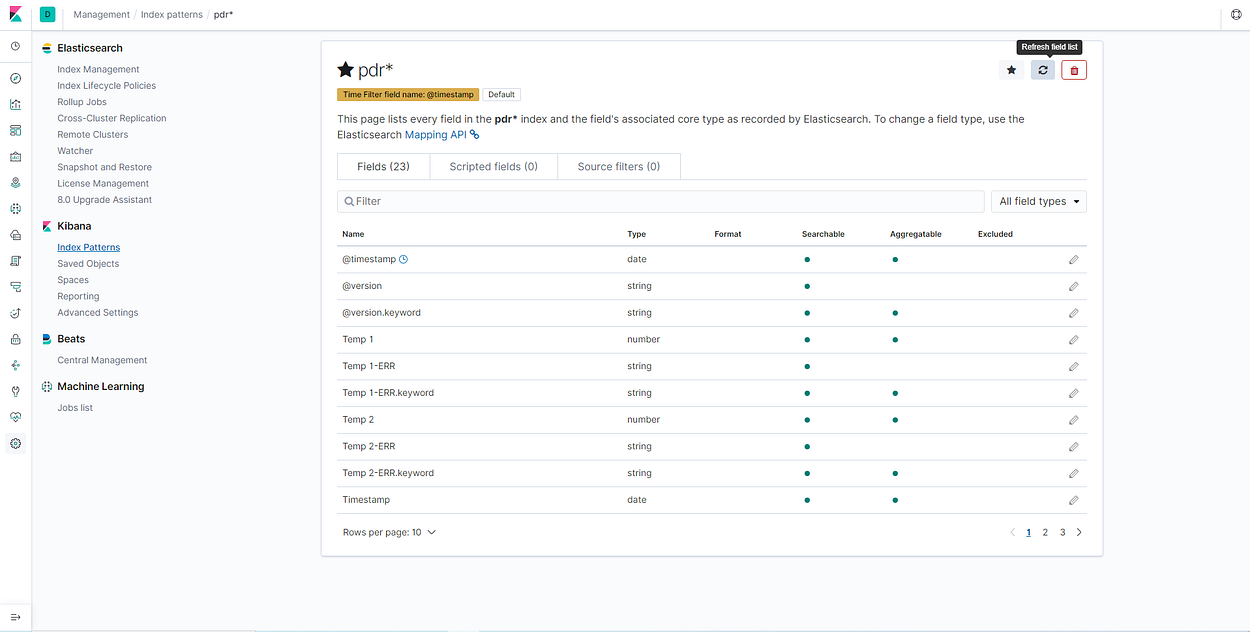 [/vc_column_text][vc_empty_space][vc_column_text]
The fields listed in the table should then match the fields you expected to be imported and match that of the Elasticsearch index pattern.
Discover
The ‘Discover’ page is the best place to confirm that the data you intended to publish is being aggregated by Elasticsearch. Here you can add metrics to the window and choose a date range in order to scroll through your data. It will show the number of events during the selected time period and confirm that your system is ready to be analyzed. In the field selection area on the left, you’ll want to confirm that the tag names you defined in the PDR are showing up here. If not, you’ll want to debug your configuration file.
[/vc_column_text][vc_empty_space][vc_column_text]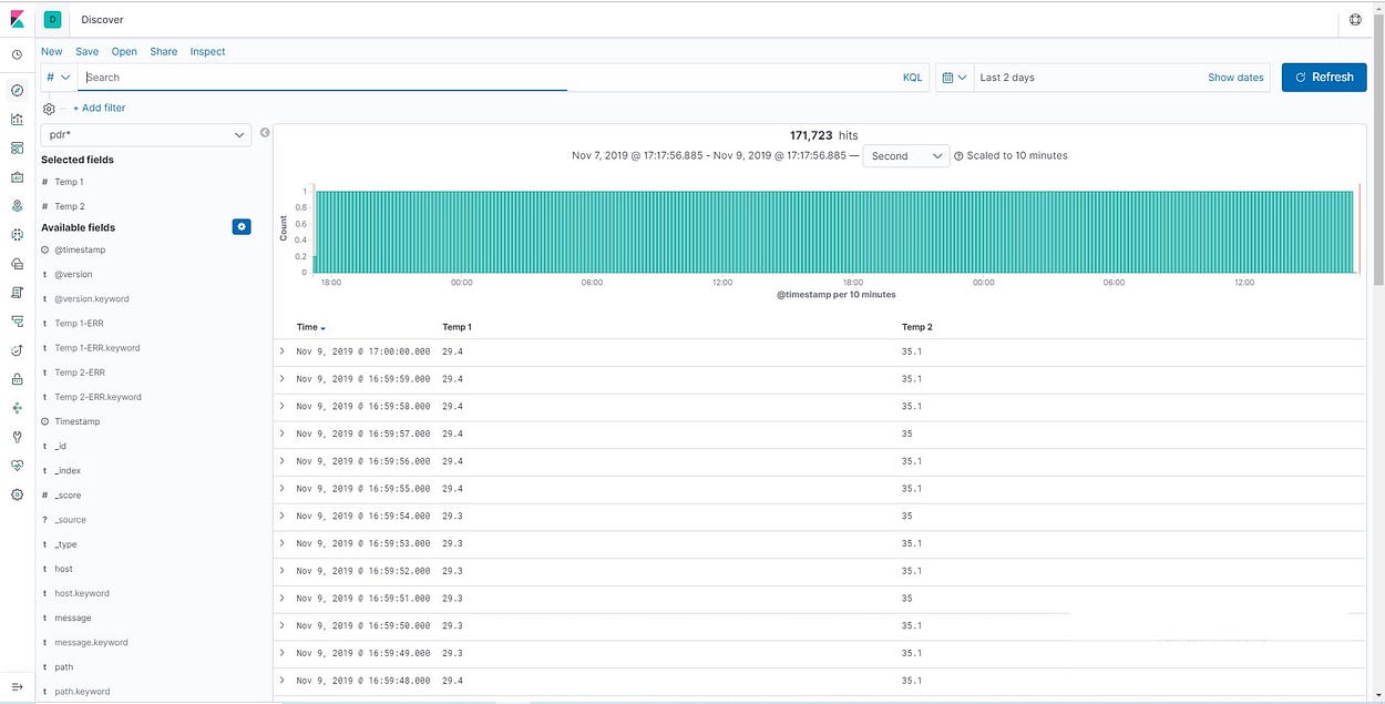 [/vc_column_text][vc_empty_space][vc_column_text]
Visualize
After confirming that your data is in Elasticsearch successfully, the next interesting step would be to use the visualize tab to create a simple visual of your data over time. Click the visualize icon on the navigation bar. It’s the third one down from the top and looks like a line chart.
[/vc_column_text][vc_empty_space][vc_column_text]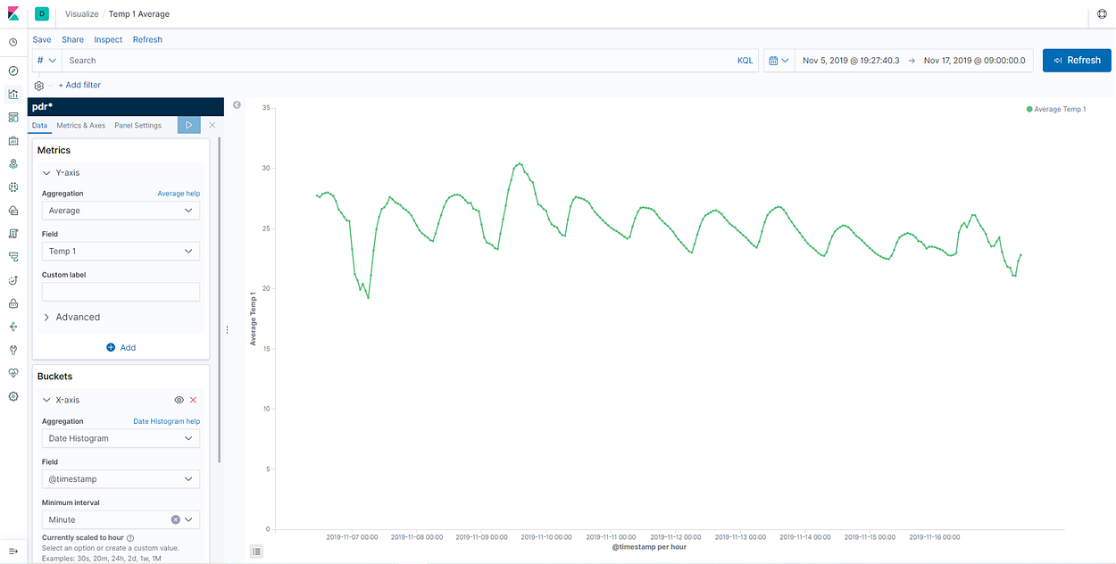 [/vc_column_text][vc_empty_space][vc_column_text]
As shown in the plot above, you’ll want to select ‘Date Histogram’ under the buckets (X axis) selection. The minimum interval represents the smallest interval of data to be rendered on screen. The X-axis field should be @timestamp. To get values on the plot, you’ll need to add a metric, an aggregation type and a field to plot. Once that is complete, the calendar widget in the top right will allow you to change the date range visualized. Click refresh to update the window.
Using this visualize tab, we can create widgets that can help visualize our industrial sensor data while also being able to visualize the other Elasticsearch data simultaneously. Using the Elastic tools, network traffic, device logs and application logs can all be aggregated and then mapped onto the industrial network or process data. The visualization and discover tools in Kibana can then be used to gain greater insight into the operation metrics of a business. They can provide the basic functionality of SCADA analytics system with the added value of mapping that data to business and IT data.
Machine Learning
While basic data visualization tools through this architecture provide some insights, the advanced features of Elasticsearch and Kibana can generate a host of new value. In order to follow these examples, you’ll need to enable a 30 day trial or purchase an Elastic license.
A good place to start in the Machine Learning tab is the Data Visualizer tab. This will provide an analysis like the one below, giving you an overview of the trend of your data over time.
[/vc_column_text][vc_empty_space][vc_column_text]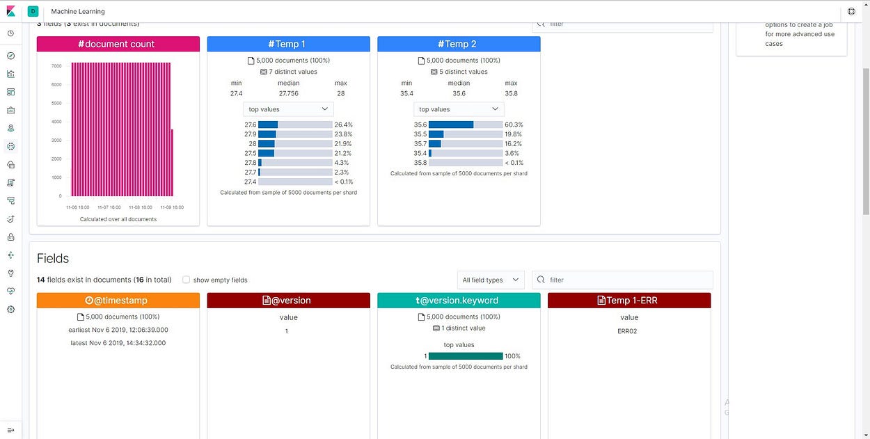 [/vc_column_text][vc_empty_space][vc_column_text]
To get started with the full machine learning feature, go to the ‘Machine Learning’ tab in Kibana. There you’ll need to click ‘Create new job.’ This function reads the data in Elasticsearch and trains a machine learning model. You’ll need to select the ‘PDR’ index. You’ll then be able to select the type of machine learning job to create. For this example, we’ll create a simple ‘Single metric’ machine learning job.
[/vc_column_text][vc_empty_space][vc_column_text]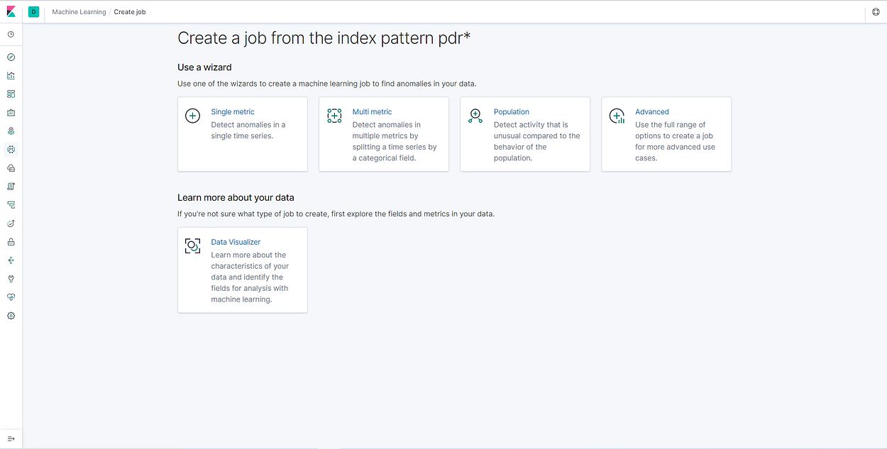 [/vc_column_text][vc_empty_space][vc_column_text]
The next screen will walk you through the steps to build the machine learning model. The first step is to select a range of data to train the model on. This configuration is meant to tell the machine learning model which data is behaving as expected. The machine learning anomaly detection will then predict if a new data point is an outlier based on that model. This training configuration will vary based on the application. For example, if you’d like to determine if a short/high frequency response is anomalous, you should select a short time range and a range in which the metric is behaving as expected. If you’d like to determine whether a metric is following a long term trend, e.g. power consumption, you should select a long time duration, perhaps a week in which the curve is behaving as expected or ‘normally.’ For this range, I selected about 2 days of temperature data.
[/vc_column_text][vc_empty_space][vc_column_text]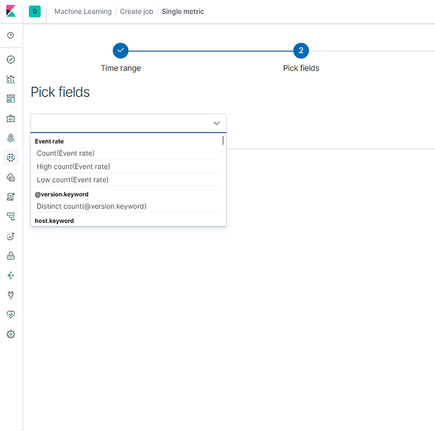 [/vc_column_text][vc_empty_space][vc_column_text]
Next, in the ‘Pick Fields’ selection, you’ll want to select the metric that you’d like to monitor. For my example, I added ‘Temp 1’ mean. The bucket span at the bottom enables you to fine tune the model time range and analysis.
After validating and running the job, Kibana will run the algorithm and provide the output as shown below.
[/vc_column_text][vc_empty_space][vc_column_text]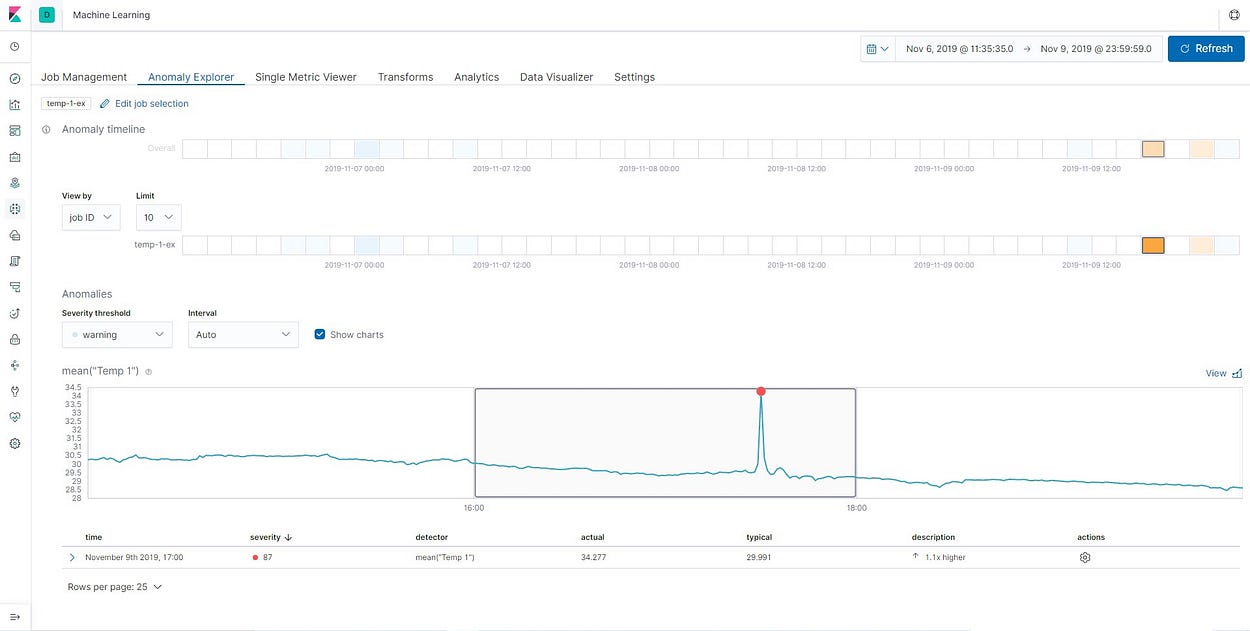 [/vc_column_text][vc_empty_space][vc_column_text]
In the ‘Anomaly Explorer’ tab, Kibana gives a timeline view to anomalies and their associated severity level. In the graphic above, you can see a high severity anomaly which corresponds exactly with a test I ran by temporarily warming temperature sensor 1. There are also some less severe anomalies detected. Notes can be taken on these anomalies for later reference.
Along with monitoring your metrics for anomalies, the machine learning feature can predict trends of the metric into the future using the forecasting feature.
[/vc_column_text][vc_empty_space][vc_column_text] [/vc_column_text][vc_empty_space][vc_column_text]
Using these two features, we can get a sense of how the process is performing. For operators, using alarms and predetermined set points, basic anomalies are usually already known. Combined with these tools, operators can get a sense of when their system is not performing normally and determine the conditions under which these anomalies are generated. Machine learning can help determine new and unknown error cases and alarm conditions. With the prediction utility, operators can then determine possible remedies for these conditions and improve system performance.
By combining this data with business and IT data, a whole host of new value can be gained. Some interesting questions that these tools could help answer are
- How is or was my industrial system affected by a cyber security attack?
- Does the quality of my electric utility have an adverse affect on my process?
- Are my devices operating the same as when I installed them and should they be replaced?
- Are there wireless or wired network devices which are adversely affecting my process and business output?
- Are there optimizations of my process which can be performed to more closely follow my customers’ ordering schedule?
These are just a few ideas for questions that could be answered by machine learning technology being applied across an industrial business’s data sources. One of the most interesting applications of this technology is the monitoring of endpoint devices and providing additional maintenance services or an online monitoring portal for end customers. Bringing industrial data sets into the hands of IT and Web developers, such as this example, has big potential for new business models and cost savings.
While the application opportunities are endless for big data analytics applied to industrial businesses, I am most excited for the added collaboration these technologies are bound to bring. I look forward to the future where more operators, business professionals, and IT personnel work together to provide new value to their business. Elasticsearch is a great technology for this collaboration. Combined with the PDR 1000, you have an intuitive and cost effective option for the next generation of industrial analytics.
[/vc_column_text][vc_separator style=”shadow”][vc_column_text]Source: https://medium.com/[/vc_column_text][/vc_column][vc_column width=”1/3″][vc_wp_text][xyz-ips snippet=”metadatatime”]
[/vc_wp_text][/vc_column][/vc_row]